Traditional neural networks (multilayer perceptron and associated feed-forward architectures) do not perform well on sequence data. Let’s take a toy problem to see this for ourselves.

Suppose we have the most basic sequence modeling problem: Given a sequence of words, predict the next word.

We can use a traditional feed-forward network if we 1-hot encoded the last \(N\) words and concatenated them to form an input vector. This is a reasonable approach, however, it precludes us to reason beyond the context provided from the past \(N-1\) words.

To get around this, we can encode the entire sequence into our vector. However, now we can’t simply concatenate each word’s 1-hot encoding because the sequence could be arbitrarily long and in this set-up the length of our vector is linear in the length of the sequence. By using the bag of words technique, we can make this \(O(V)\) instead of \(O(|S|)\) (size of our vocabulary instead of size of the sequence). The bag of words simply counts the number of occurrences of each vocabulary element in the sequence.

While this gets the size of the encoding under control, it loses all information about the ordering of the sequence.

What if we made a compromise and used a fixed-length window, but a very large one? We can assume for example that context from elements any more than 100 steps ago should not be needed when thinking about the current element.

This is a reasonable compromise, but still has the problem that the neurons that will be operating at data on one end of the sequence will never get the chance to see the information in the beginning of the sequence.

Therefore, we really do need a new architecture that is specifically designed for sequential data. At a high level, we can think about three sources of difficulty presented by sequential data:

1. For most sequential data, the length of the sequence need be a free parameter whereas feed forward networks require fixed-size inputs.
2. The order of data needs to somehow be preserved and modeled, something that FF’s don’t do well
3. In addition to preserving order, reasoning about sequential data may require a notion of memory. Meaning, when operating on \(X_i\), we may need information about \(X_{i-n}\) for some large \(n\) to arrive at the correct answer. This requires us to design the network in a way that allows a single (or a set of) neuron to both see all examples, as well as be able to have the capability to relate information from different positions in the sequence to one another.

Recurrent Neural Networks

Recurrent Neural Networks (RNNs) solve most of these problems, and give birth to more sophisticated architectures that make progress on the unsolved ones.

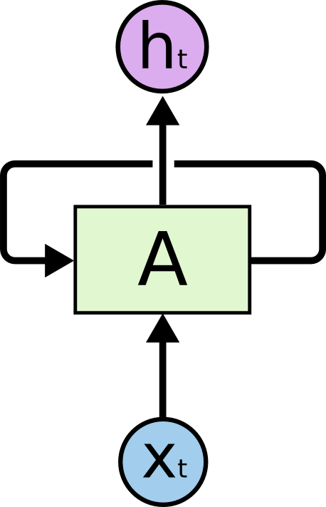
At the most basic level, at every time step, the RNN cell

• Receives an input \(x_t\)
• Computes an output \(y_t\)
• Updates its internal state \(h_t = f_W(h_{t-1}, x_t)\) using the previous state and the current input, and a function parameterized by \(W\).

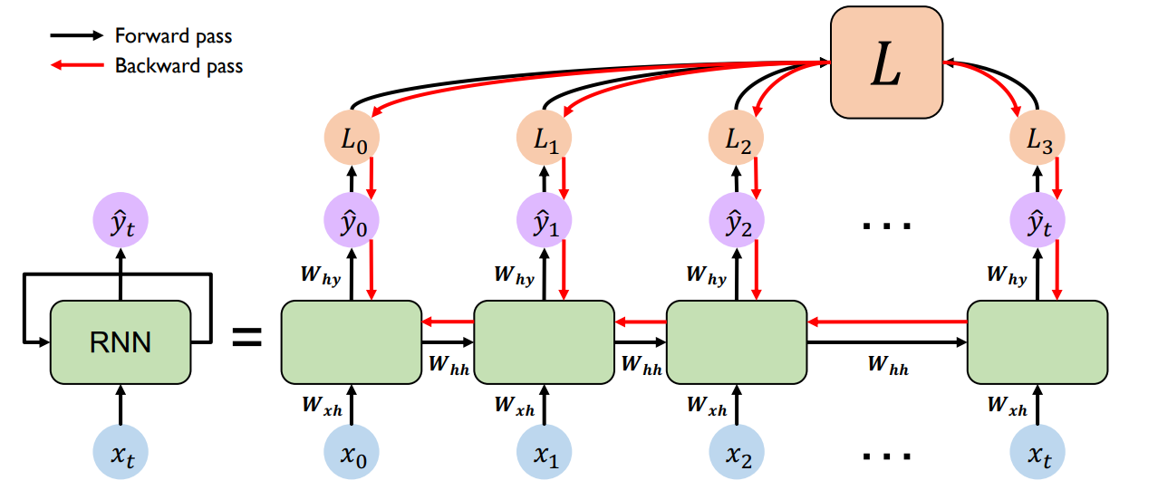
It is important to note that this function and weights are shared among all instances of this cell, and that this recurrence (reliance of \(h_t\) on \(h_{t-1}\)) can be unrolled across time, forming the following topology.

We train these cells via an algorithm called backpropogation through time (BPTT), depicted below.

From the figure, we see that the total loss is \(L = L(\Theta) = \sum_t L_t(\Theta)\). We can compute the gradient of the loss with respect to each parameter: \(\frac{\partial L}{\partial P} = \sum_t \frac{\partial L_t}{\partial P}\)

Let’s try computing the gradients for a single timestep, \(t_3\). Applying the chain rule to \(\frac{\partial L_3}{\partial W_{xh}}\) we get \(\frac{\partial L_3}{\partial y_3}\frac{\partial y_3}{\partial W_{xh}}\).

Remember that \(y_t = W_{hy}h_t\) where \(h_t = tanh(W_{hh}h_{t-1} + W_{hx}x_t)\).

Unrolling this one more time and putting it together, we get \(y_t = W_{hy}(tanh(W_{hh}h_{t-1} + W_{hx}x_t)) = W_{hy}(tanh(W_{hh}(tanh(W_{hh}h_{t-2} + W_{hx}x_t)) + W_{hx}x_t))\).

The problem here is that not only does \(y_t\) directly depend on \(W_{xh}\) in timestep \(t\), but it’s also dependent on all the previous cells through the propogation of the hidden state of the previous cell (which transitively depends on all previous \(W_{hx}\).

This means the calculation of gradients is going to involve on the order of \(N\) matrix multiplies and nonlinear activations for a network with \(N\) unrolled cells. This is problematic because the gradients are likely to explode to large numbers or vanish to zeros, due to the high number of successive multiplications by the same set of non-unit factors.

This means that we cannot effectively learn long-term dependencies - the further back we try include in our context, the more likely that the gradients explode or vanish.

There are a number of ways to get around this problem: we can be clever about the initialization of our parameters or use activation functions that make explosion/vanishing unlikely, for example using ReLU instead of Sigmoid or hyperbolic tangent since ReLU yields unit derivative for positive inputs. However, that’s still not a thorough fix.

Long-Short Term Memory

The mitigation for this situation is a new architecture, one that allows information to flow through the network for arbitrarily long periods of timesteps without having to flow through expensive gradient computations. One such network architecture is Long-Short Term Memory or LSTM networks.

There are two important distinctions about LSTMs:

• They maintain separate cell state from what is outputted in order to isolate the complex calculations needed to update the cell’s state from what will be needed to calculate gradients for BPTT
• They add or remove information to the cell’s state through structures called gates (similar to the ideas of gates in Digital Logic Design)

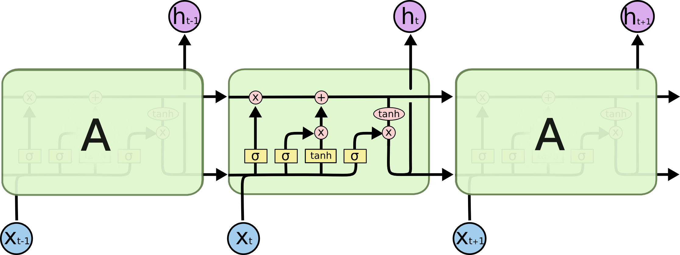
Let’s take a quick look at the schema of an LSTM cell:

As mentioned before, the cells keep an internal state \(c_t\) that they cram information into. At every time step, there are two main steps that LSTM cells do:

• Update its internal state
• Generate an output based on the cell state

Update

Updating itself is done in two steps: forget and add.

Forget

Forget is a sigmoid layer that looks at the previous state and current input and outputs a number between 0 and 1 for each bit in the state which represents the portion of it that should be kept. \(f_t = \sigma(W_f \dot [h_{t-1}, x_t] + b_f)\)

Add

Now, we have to decide what to add to our state. This is done in two steps: candidate generation and candidate selection, where candidates are elements of the state and input vectors concatenated.

Candidate generation

\[\tilde{C}_t = tanh(W_C \dot [h_{t-1}, x_t] + b_C)\]

Candidate selection (input gate)

\[i_t = \sigma(W_i \dot [h_{t-1}, x_t] + b_i)\]

Now we simply have to use these quantities to update the cell by forgetting and adding the appropriate information.

\[C_t = f_t*C_{t-1} + i_t*\tilde{C}_t\]

Output

Now that we have our updated state, we transform and gate it to produce the final cell output.

Output gate \(o_t = \sigma(W_o \dot [h_{t-1},x_t] + b_o)\)

Transform and apply gate \(h_t = o_t * tanh(C_t)\)

Wrap-up

Notice how in this formulation, gradients of \(C_t\) can flow through the top of the cell unaffected by the heavy computation going on local to each cell. This was the main motivation behind LSTMs, and why they allow networks to reason using long-term dependencies.

It’s worth noting that there are many variants of LSTM cells, all implementing the same idea with slightly different mechanics, ex. via adding peephole connections or coupling the forget and input gates more closely than we have done.

A popular variant of LSTM cells is Gated Recurrent Unit (GRU) cells. It works by combining the update and forget gate, and merging the cell state and hidden state (\(c_t\) and \(h_t\)) among other changes. It is worth noting that GRU cells are a bit more computationally inexpensive and thus are used widely in practice.

Please check out Chris Olah’s blog for more explanations and awesome graphics (some of which I’ve used here) and MIT’s intro course for Deep Learning for more reading and tutorials on these topics.